|
Huashi 24 GHz Radar - RF Engineering Notes: From Requirement Targets to Production ParametersField notes on a 24 GHz ground radar: three requirement tiers, link budget, three architecture grades, front-end selection, frequency source and sampling, FPGA and power, schematic and PCB, staged testing, array calibration, and the parameter package required for domestic second-sourcing. Every number here tries to carry its measurement plane and its conditions — because “19 dBm” without a reference plane is not comparable engineering. Key points
1. Requirement Quantification: What Counts as PassedThree requirement tiers and a starter calculationThe first requirement table cannot say only “long range, high accuracy, fully domestic”. Put numbers on paper. An internal review should list three versions: a contract gate, a delivery commitment, and a design internal control set. The contract gate decides whether the system can be accepted; the delivery commitment keeps margin for mistakes and ageing; the internal control set leaves room for device spread, temperature drift, assembly tolerance and instrument uncertainty. Do not blend the three. If range R0 is the discussion point, do not convert it straight into transmit power. First fix the target RCS distribution, detection probability Pd, false-alarm probability Pfa, target velocity range, terrain clutter, antenna height and available integration time. For an FMCW link, start with the receiver noise floor: N = -174 dBm/Hz + 10log10(ENBW) + NF With a 1 MHz noise bandwidth and a 6 dB receiver noise figure, thermal noise is about -108 dBm; if a single range-Doppler cell needs 13 dB SNR ahead of detection, the usable signal at the receiver is about -95 dBm. Close that against two-way path loss, antenna gain, target RCS and processing losses. Do not write “the FFT has 1024 points, so 30 dB gain”: coherent integration tops out near 30 dB, and windowing, range migration, phase noise and calibration residuals all take a bite out of it. Start range resolution with ΔR = c/(2B). At B = 15 MHz that is about 10 m, at 30 MHz about 5 m, at 150 MHz about 1 m — but 150 MHz also loads the ADC, clock jitter, PA response, antenna match and dechirp linearity. On the IF side, fIF = 2RB/(cT): with R = 3 km, B = 30 MHz and sweep time T = 1 ms, the Doppler-free beat is about 0.6 MHz; under the same conditions with T = 100 μs it is about 6 MHz. The first case is easy for the ADC but harsher on sweep linearity, frame time and the near-range blind zone; the second is the other way round. Resolution, maximum range, first-report time and velocity ambiguity must be solved together, not picked one at a time because one of them looks good. On angle, if 120° azimuth coverage is required, ask first whether that is mechanical scanning, electronic scanning or a multi-face array. Take a uniform linear array with about 0.5λ spacing: scanning to ±60° still has to account for element pattern roll-off and mutual coupling; if angle error below 1° is required across the full field of view, a 1° beam step will not get you there. For an engineering prototype, set the element amplitude/phase calibration residual target at amplitude RMS ≤ 0.3 dB and phase RMS ≤ 3°. That is the starting point of the array error budget; the final value must be derived from the beam pattern and known-angle targets. Requirement review table: ask by dimension, not by page count
Radar equation and the “stated assumptions”Write the radar equation in a form a review board can check. Received power is: Pr = Pt + Gt + Gr + 10log10(σ) - 20log10(R) - 20log10(4π/λ) - Ltotal Work in dB/dBm. After dechirp, also write the receiver noise floor as N = -174 dBm/Hz + 10log10(ENBW) + NF, then subtract processing gain, window loss, range/Doppler migration loss, clutter and calibration residuals. The biggest trap is treating FFT size as SNR gain: coherent integration approaches 10log10(N), non-coherent integration falls below it, and windowing, phase noise and range migration keep eating the rest. Present the assumptions explicitly — target RCS σ0, range R0, antenna gain G0, total loss L0, giving link margin M — but never dress an assumption up as a measured customer specification. Red flags are the obvious ones: quoting chip output as port power; an operating temperature of only -40 to +70 °C where the product needs more; price and lead time kept secret. Green lights are: requirements frozen, link margin ≥ 6 dB, thermal margin ≥ 10%, power margin ≥ 20%, at least one validated primary source and one board-validated second source for every critical part, and a test method plus acceptance instrument for every specification. 2. Three Routes Side by Side: a Demo Runs Fast, a Prototype Must Scale, Production Must Be ServiceableStarting parameters for the three gradesVersion A aims to get RF, ADC and the host GUI running within four weeks, and does not undertake to prove long range. Pick a single-chip 1T1R/1T2R device inside an authorized 24 GHz sub-band, with 0 to 10 dBm at the chip output, a 2×2 or a 1×4 on-board microstrip array, and 8 to 12 dBi estimated array gain; do not raise EIRP on your own without authorization. The receive chain should not stack external LNAs yet — keep an on-board coaxial loopback and a controllable attenuator. Test targets might read: bandwidth in three steps of 10/30/100 MHz, ADC at 40/125 MSPS effective, at least 256 MB of raw IQ per frame, two hours of continuous capture without data loss; spectrum, phase noise and power all per the official chip datasheet. What Version A should test is not maximum range but short-range fixed-target stability. Put a corner reflector or metal sphere at authorized test points of 30 m, 100 m and 300 m, record 1000 frames at each, and compute mean range, standard deviation, missed detections and phase drift. If 300 m images stably but the 3 km field test drops out the moment you power up, the problem is most likely link, clutter and algorithm — not code that cannot draw an FFT. Version B should be 2 transmit and 4 receive, with four receive channels in parallel and time-multiplexed transmission, avoiding the supply, intermodulation and thermal peaks of several PAs running at once. If each of the four receive IFs tops out at 10 MHz, a 65 MSPS ADC will do; if each reaches 40 MHz, move to 125 MSPS or above. Channel-consistency targets can start at amplitude ±0.5 dB, phase ±5°, and inter-channel sampling clock skew ≤ 200 ps, tightening after a single-station calibration to amplitude RMS 0.2 dB and phase RMS 2°. These are internal design targets, not chip marketing numbers. Lay out each receive chain as “RF limiter/switch - bandpass - LNA - attenuator - mixer/downconversion - IF filter - ADC”. Every additional 0.5 dB of front-end loss degrades system noise figure by nearly 0.5 dB, all else equal, so more protection devices are not automatically safer. With a 0.4 dB switch, a 1.0 dB filter and 0.3 dB of trace and connector loss ahead of the LNA you already have 1.7 dB; at that point choosing an LNA with 1.2 dB NF is far less valuable than cutting front-end loss from 1.7 dB to 0.8 dB. Version C should first bring up a single 1T1R RF branch. Drive up- and down-conversion from a common LO: the transmit branch runs modulation/conversion - driver - PA - directional coupler - filter - antenna; the receive branch runs limiter - preselection - LNA - image rejection - mixer - IF amplifier - anti-aliasing - ADC. Do a 50 Ω fixture-level test first, then a four-channel array. Size the PA from backed-off power: if the antenna port needs 23 dBm average and the switch, filter and feed together lose 1.5 dB, the PA port must deliver 24.5 dBm; with 6 dB linear back-off, the PA needs at least about 30.5 dBm P1dB. That simple addition prevents promising 23 dBm linear output from a device with 24 dBm saturation. At equal power, antenna gain is cheaper than PA power. All else unchanged, 3 dB more antenna gain is equivalent to 3 dB more on the transmit or receive side; but 3 dB of antenna gain usually buys a narrower beam, a larger aperture and tighter assembly. A production plan must add up antenna gain, scan loss, radome loss, PA back-off, supply efficiency and heat dissipation together — not just compare price per watt of PA. Three grades, three different questionsGrade A, the fast demo, uses a single 24 GHz SoC straight into a microstrip array, with an FPGA or MCU doing configuration, capture and host transfer only. Huashi S3KM111L is published as 1T1R with up to 1 GHz sweep range, 12 dBm transmit, 10.5 dB noise figure, -97 dBc/Hz at 1 MHz, a 16-bit 2.5 MSPS throughput ADC, FFT/CFAR hardware acceleration and -40 to 105 °C junction temperature; Huashi RC2412 is 1T2R, 23.5 to 25 GHz, 5 dBm per channel, 15 dB receive NF, -100 dBc/Hz at 1 MHz with dual ADCs; Huashi RS2111 is a 1T1R, 10 dBm, roughly 10 dB NF, -105 dBc/Hz at 1 MHz low-power sensing SoC. Parts like these let a team validate antenna, waveform, algorithm and data interface quickly, but they cannot prove a long-range link. Grade B, the scalable engineering prototype, is best built around a 2T4R device such as Huashi SRK2401A/SRK2402. The published Huashi page lists SRK2401A as 2T4R, 9 dBm, 29 dB receive gain, 9 dB NF, -8 dBm P1dB, -103 dBc/Hz at 1 MHz, 3.3 V/435 mA, QFN56; another public page lists SRK2402 as 24.00 to 24.25 GHz, 2T4R, with 29 dB conversion gain, 9 dB NF, -14 dBm input P1dB, 9 dBm transmit, SPI control, 3.3 V/390 mA, 7×7 mm QFN and -40 to 125 °C. The two pages quote P1dB differently for the same family — a reminder that identical packages and similar names do not mean data can be inherited. Go by the formal datasheet revision, test conditions and ordering suffix. Grade B can add a limiter/switch, LNA, bandpass, controllable attenuator and board loopback on every channel; transmit time-multiplexed, receive four channels in parallel, validate calibration and the array first, and only then decide whether to add an external PA. Grade C, the long-range / production candidate, does not worship single-chip power; it uses multi-chip synchronization or a discrete common-source architecture. Recommended signal flow: low-phase-noise reference - integer/fractional-N PLL and loop filter - 24 GHz LO distribution - I/Q modulation or direct FMCW generation - driver - PA - coupled detector - T/R or antenna switch - receive limiter - LNA - image-rejection filter - variable gain - I/Q demodulation/dechirp - anti-alias filter - ADC - FPGA. For 4T8R or larger, prefer a common LO tree, programmable phase shift/delay and multi-chip sync; settle clock, power and LO distribution before the digital algorithm. For “domestic, manufacturable, cost-effective”, Grade C does not start by stacking GaN — it first uses link margin to prove how much EIRP is needed, then compares the cost of more antenna gain, less loss, longer dwell and more PA.
3. The 24 GHz Front End: Define the Measurement Plane FirstWhich connector or pad is the measurement planeThe first front-end selection question is “at which connector or pad is the measurement plane”. The published Huashi ARS-2401 module gives 24 to 24.25 GHz, 20 dBm EIRP, 15.5 to 26.5 dB receive gain, 12 dB SSB NF, -26 dBm input P1dB, 3.3 V at 47 to 57 mA and an 80°×32° on-board antenna. That suits a low-cost module survey, but EIRP already includes antenna gain and cannot be compared with bare-chip PA port power; the -26 dBm input P1dB also says front-end protection is not optional near strong close-in reflections. Huashi ARS-2412 is published as one transmit and two receive, 80°×32°, 10 dBi, 3.3 V, 150 to 270 mA and -40 to 105 °C — still usable as a “mature module reference”, but no substitute for a manufacturability assessment of a bare-chip design. Choose the PA by backed-off linear powerChoose a PA by backed-off linear power, not by saturated power in the headline. The published Huashi DPA8-24-34-3142 page gives 24 to 34 GHz, 14 dB nominal gain, 24 dBm P1dB, 29 dBm saturation, +12 V/1 A, 2.92-K and -40 to +70 °C; enough for one engineering demo, not enough for a production commitment. Its own table shows about 15.65 dB S21 and 27.8 dBm P1dB near 24 GHz, which differs from the “14 dB/24 dBm” summary — so formal design must use test reports tied to the ordered lot and worst-case values, not typical curves. If the system is linear FMCW rather than pure CW, back the final stage off 3 to 6 dB from P1dB; needing 23 dBm average at the port means looking for 26 to 29 dBm P1dB and at least 13 dB in-band gain, while accounting for duty cycle, thermal resistance, harmonics and load mismatch. The LNA’s first job is noise; its second job is survivalReasonable starting values: LNA NF ≤ 2.0 dB, gain 18 to 22 dB, input P1dB ≥ -10 dBm, OIP3 ≥ 5 dBm, with a low-loss limiter or RF switch ahead so that the LNA input stays below its damage and compression limits at maximum expected leakage and close-in reflection. Friis shows that with 20 dB LNA gain and 1.8 dB NF, a following mixer at 10 dB NF and 3 dB of passive loss contribute very little at the input; but if the filter and switch ahead of the LNA already cost 2 dB, system NF degrades by nearly 2 dB, so protective elements cannot be stacked without limit. Mixing, filtering and image rejectionThe decisive mixer and filter specifications are image rejection, LO leakage and group delay. Published Huashi HH-MX560 data gives RF/LO 21 to 40 GHz, IF DC to 18 GHz, 8 dB typical conversion loss, 13 dBm LO drive, 12 dBm RF input P1dB, 45 dB LO-RF/LO-IF isolation, a chip range of -55 to 125 °C, 1.192×0.822×0.1 mm, with AuSn or conductive-epoxy die attach, 25 μm gold wire and bond wires shorter than 250 μm. Huashi DM8-6-26G-9199 is a 6 to 26 GHz double-balanced passive mixer module, about 8 to 9 dB loss near 24 GHz, 11 dBm RF P1dB, 20 dBm IIP3, but its operating temperature tops out at +65 °C and RoHS status must be confirmed per lot — better for a lab fixture than for an unqualified outdoor product. For filters, start with a 3 to 5 pole LTCC, cavity or microstrip bandpass over 23.9 to 24.3 GHz or the authorized sub-band, 1.5 dB or less insertion loss, out-of-band rejection allocated by need; measure group-delay ripple before production, because it converts into range sidelobes with the sweep slope. Port accounting, receive budget and filter starting valuesAny “19 dBm” without a stated measurement plane is not comparable engineering. A worked receive budget: 0.8 dB loss from antenna to the LNA, LNA gain 20 dB with 1.8 dB NF, then 2 dB filter loss, 8 dB mixer conversion loss and a 5 dB NF IF amplifier. By Friis, after the 1.8 dB front-end loss the second 2 dB stage contributes about 0.03 dB and the 8 dB mixer about 0.31 dB; total NF lands around 2.2 to 2.5 dB, with the exact value depending on the gain distribution and measured parts. Cutting the post-LNA filter from 2 dB to 1 dB improves total NF by only about 0.1 dB but may improve blocking significantly — argue that trade with numbers. Do not write image rejection as a bare “60 dB”. State input and output frequencies, LO frequency, power, temperature, bandwidth and measurement resolution. Internal control might start at image rejection ≥ 45 dBc, LO leakage ≤ -20 dBm (measured at the mixer RF port) and double-sideband noise difference ≤ 1 dB; tighten if the NF target and blocking conditions demand it. With less than 8 to 10 dBm of LO drive, conversion loss and IIP3 may degrade noticeably, while excessive LO increases leakage and radiated LO, so sweep ±2 dB around the recommended value. 4. Frequency Source, Sampling and FPGA: the Radar’s MetronomeLinearity, jitter and ADC test conditionsConstrain FMCW linearity with three metrics at once: in-band phase noise, chirp frequency error and residual phase error. With 30 MHz bandwidth over 1 ms the ideal slope is 30 GHz/s. If range sidelobes must not visibly degrade from linearity, look first at how the PA, VCO tuning and supply disturb the slope; do not “fix” it in the algorithm first. Production BITE can inject a fixed delay into the transmit coupled path, compute the phase residual of each chirp, and generate a pre-distortion table per board. Use 16 to 64 control points, one set each at -40, 25 and 85 °C; more points is not better — too dense and the table learns the measurement noise. Clock jitter follows SNRjitter = -20log10(2π·fin·tj). At 100 MHz input with a 70 dB jitter-limited SNR, tj must be about 0.50 ps RMS; at 200 MHz, about 0.25 ps. If the ADC aperture jitter is already 150 fs, clock buffering 200 fs and the PLL 300 fs, the root-sum-square is about 390 fs, leaving little for board crosstalk and supply noise. Convert a clock chip’s “typical phase noise” into integrated jitter over the target offset range — do not judge it by a single -160 dBc/Hz point far from the carrier. Do not test an ADC on full-scale SNR alone. Run at least four cases: a low-frequency sine, a near-Nyquist sine, two tones and zero input. The low-frequency sine shows ENOB, near-Nyquist shows aperture jitter and drive, two tones show SFDR and intermodulation, zero input shows offset, code density and supply coupling. Synchronize four ADCs with the same digital ramp and measure inter-channel delay; if 200 ps is required, one sample period at 65 MSPS is already about 15.4 ns, so the digital side must do deterministic delay calibration rather than rely on “roughly equal-length” traces. A 24 GHz VCO’s phase noise cannot be judged outside the PLL loop and the tuning linearity. Published Huashi HGC592-12F material describes a GaAs VCO covering 15 to 21 GHz with W2120 and 15 to 24 GHz with M470, +12 dBm output, -87 dBc/Hz SSB at 100 kHz offset, +5 V/52 mA, 0.3 MHz/°C drift, a 1.5×1.5 mm die requiring an external varactor, 0 to 20 V tuning and wire assembly. It shows a domestic process can supply candidates; it does not prove that a complete 24 GHz chirp meets linearity and production consistency. With a multiplier architecture, remember that ideal N-times multiplication degrades phase noise by 20log10(N): 12 to 24 GHz costs 6 dB in theory, and multiplier excess noise, supply and amplifiers make it worse. With a fundamental VCO, the problems are wide tuning sensitivity, Kvco variation and analog pre-distortion. The ADC for four receive channels is another critical part. One Huashi four-channel ADC comes in a QFN package with a datasheet, EVB guide and compliance documents, a strong candidate for four receive channels, though purchasing status still has to be confirmed through the factory or an authorized channel. SD9650-65 is listed as ACTIVE on an authorized distribution platform, dual 16-bit 65 MSPS, 9×9 mm 64-LFCSP, industrial grade — a candidate for a low-bandwidth dechirp path, but platform parameters do not replace a full-temperature factory datasheet. A DAC is not mandatory in every FMCW designIf the PLL generates the chirp directly, the DAC only handles VCO coarse tuning, power control or calibration; with an RFDAC/DDS upconversion, the DAC decides image, spurious and waveform flexibility. Huashi DAC2169-1000 is published as dual 16-bit, 1 GSPS, 2×/4×/8× interpolation, complex modulation, multi-chip sync and auxiliary DAC, but the complete factory datasheet, price and stock still need confirmation, so it belongs on an evaluation list, not in a frozen BOM. Another Huashi four-channel 16-bit 2.4 GSPS DAC offers DUC and 8-lane JESD204B, SFDR > 72 dBc at 180 MHz, under 3 W at 1.6 GSPS, a 12×12 mm package and -55 to 125 °C, but the public page gives no orderable part number, so it cannot enter a BOM either. 5. FPGA, Clocks, Power and Interfaces: Not RF on Paper, All RF in the EndRough power estimate and supply isolationDesign the 28 V input for maximum input, start-up inrush and PA pulse peaks. As a rough case — 12 V/1.5 A for the PA, 5 V/1 A for the RF chain, 1.0 V/3 A FPGA core, 3.3 V/1 A, and 1 A for interfaces and miscellaneous — steady-state input power is about 18 + 5 + 3 + 3.3 W plus losses, already close to 35 W; with 20% PA duty cycle and higher peak current, the DC/DC and input fuse still have to be sized for peak loop capability. At the input, add reverse protection, TVS, common-mode choke, differential-mode π filter and soft start, and write the surge test level, source impedance and test waveform into the acceptance record. Never share one long thin trace between PA and LNA supplies. Follow the datasheet power-up sequence for the PA gate/bias, add local 100 pF, 1 nF, 0.1 μF and 10 μF decoupling at the drain in layers, with return vias close to the device; isolate the LNA supply with RC or LC, keeping the corner away from control loops and low-frequency oscillation. Use a low-noise LDO for the PLL charge pump: it draws only a few milliamps, but its noise modulates the VCO directly. Sequence FPGA rails with a supervisor, and latch undervoltage, power loss, overtemperature, PLL unlock and ADC overflow as faults. Inside the board, run Gigabit Ethernet as RGMII or SGMII consistently with the PHY choice, converting to fiber for long outdoor runs; specify RS-485 node count, 120 Ω termination, common-mode range and fail-safe bias. If multi-station range consistency within 30 m equivalent is required, 100 ns of timing error alone corresponds to about 30 m of one-way path — distinguish “network time as displayed” from “the instant of RF sampling”. Within a station, the sampling clock is the reference; between stations use a GNSS-disciplined oscillator or PTP, and calibrate antenna feed, cable and algorithm latency together. Calculate FPGA throughput before choosing a vendor. With four low-IF receive ADCs at 16 bits and 65 MSPS, raw data is about 4.16 Gbit/s; four channels about 16.7 Gbit/s, before control, DDR buffering, FFT/CFAR and Ethernet overhead. Published Huashi JESD204B IP guidance states up to 8 lanes per IP, Subclass 1 only, with a GW5AT 8-channel TX+RX example using roughly 12,816 registers, 13,612 LUTs, 3,402 ALUs and several memory blocks, and stresses a stable low-jitter reference clock and SYSREF. The Huashi Titan II family lists PG2T70H/160H/390H/390HX with HSST up to 12.5 Gbps per lane, 6+6, 8+8 and 10+10 lane options, DDR4 and complete hardware design material. An entry design can therefore use something like PG2T70H to carry four 125 MSPS ADCs with processing headroom; eight receive channels, wideband JESD or multi-GSPS RFDAC means more lanes and larger memory. Confirm speed grade, JESD IP licensing, production tool version and industrial/military temperature ordering codes with the vendor. For the clock tree, use a 10 MHz OCXO or a high-stability TCXO as the system reference: close-in phase noise is set by the 24 GHz PLL loop, far-out and long-term drift by the reference; give ADC/DAC/JESD their own low-jitter PLL or clock distributor, and never share an unevaluated ordinary crystal between the FPGA reference and the RF sampling clock. Production designs must support BITE for missing reference, PLL unlock, abnormal clock amplitude and SYSREF repeatability. Do not write “choose a low-phase-noise clock chip” without a measurement plane: budget phase noise and spurious at the reference input, PLL phase detector, VCO tuning, LO buffer and ADC clock separately, and cross-correlate on a common time base. Power follows a three-stage structure: bus, point of load, then local cleanup. Take 28 V or a 48 V input through reverse protection, surge, common/differential filtering and ideal diodes, then generate 12 V for the PA, 5 V for RF MMICs and some clocks, 3.3 V for ADC and interfaces, and 1.8/1.0/0.85 V for FPGA and DDR. If PA transient current is about 1 A, size the bus, decoupling and heatsink for pulse power rather than average power; sequence and supervise FPGA rails, converter analog rails and PLL supplies. Rather than forcing a single “radar PMIC”, a distributed domestic buck + LDO + supervisor design is more robust. Every critical rail needs voltage, current, temperature and fault latching, with at least 20% margin over worst-case input, ageing and drift. For external interfaces, use Gigabit Ethernet as the main data path, RS-485/RS-422 or CAN for low-speed control, fiber as an option for distance and lightning isolation, and GNSS/BeiDou with PTP for multi-station time alignment; prefer 2.92 mm at the 24 GHz RF port. Huashi 2.92 mm connectors are 50 Ω air-interface, DC to 40 GHz, VSWR 1.10 + 0.01f, 500 mating cycles, with vibration, shock, thermal shock, salt fog and humidity tests listed. But “intermateable with SMA” does not license casual use of ordinary SMA: mechanical wear, mode conversion and phase repeatability all damage array calibration. An outdoor unit needs a radome or sealed window, and production tests must specify torque, cable bend radius, end-face inspection and the calibration plane. 6. How to Draw the Schematic: Every Energy, Signal and Fault PathStarting dimensions for matching stubs and a stability sweepA first-pass PA output can start from a two-section “series line + shunt open stub + DC block”. At 24.15 GHz, with an equivalent microstrip wavelength of roughly 7 to 8 mm depending on laminate and boundary, start optimizing from a series line of 0.15λg ≈ 1.1 to 1.2 mm and a shunt stub of 0.10λg ≈ 0.7 to 0.8 mm, then correct with EM simulation and a VNA. Do not leave a single “matching network” black box in a production schematic: reference designators, dielectric thickness, copper weight, surface finish, reference ground and adjacent copper boundaries are all design outputs. Design anti-aliasing for the real IF. With a 10 MHz maximum IF and a 40 MSPS ADC, a 5-pole analog low-pass with an 8 MHz passband edge and ≥ 50 dB at 20 MHz is reasonable; a linear-phase FIR gives near-constant group delay but many taps, so count FPGA resources and latency separately. A dechirped signal near DC must handle PA leakage, ADC offset and 1/f noise: do not set the high-pass corner to a few hundred hertz by habit, or slow and hovering targets get attenuated. Better to estimate and subtract the static leakage digitally and keep observability near 0 Hz. The schematic must draw four separate paths: energy, information, control and health. Energy runs from input protection, DC/DC, switches and PA to the antenna; information from antenna, LNA, filter, mixer, IF, ADC to FPGA; control includes SPI/I2C, GPIO, PLL, attenuators and calibration switches; health includes coupled detection, temperature, voltage and current, LO lock and loopback. Title each sheet with its supply domain and interface direction, use unified net classes across pages, and mark PA gate/bias, LNA drain, PLL charge pump, ADC clock and SYSREF as “no auto-routing”. PA output matching does not end at 50 Ω; it transforms the device’s optimum load at the target frequency, bias and power to the antenna port. Get Γopt from vendor load-pull data or a large-signal model, then check with: Γ = (Zopt - Z0) / (Zopt + Z0) If the target port is 50 Ω, expected output 23 dBm and return loss ≥ 10 dB, reflected power is around 2.3 dBm; a real design must also survive antenna detuning and an open cable. A first pass can use a two- or three-element L network of series microstrip, shunt open stub and DC-blocking capacitor, with 0.10 to 0.25λg series and 0.05 to 0.20λg shunt as an optimization range at 24 GHz — not as final values. If you choose a low-loss high-frequency laminate, simulate with the actual Dk, copper roughness, solder mask and assembly tolerances; at 24 GHz a 1 mm trace error is already a visible phase shift. Match the LNA input for minimum noise impedance Γopt, not conjugate match, and draw a separate stability network. Reserve footprints for a series 0 Ω or small resistor and a shunt RC or stub, but production must not keep “nobody knows whether it is fitted” ghost positions. Judge small-signal stability with the Rollett factor: K > 1 and |Δ| < 1. When that fails, use a λ/4 high-impedance line with a fan-shaped capacitor, or resistive stabilization, plus 100 pF, 1 nF, 0.1 μF and appropriate damping at the supply entry. K = (1 - |S11|2 - |S22|2 + |Δ|2) / (2|S11·S22|), Δ = S11·S22 - S12·S21 Start RF supply decoupling with 100 pF + 1 nF right at the pad and 0.1 μF + 10 μF on the outer ring; use a dedicated low-leakage filter for the PLL charge pump rather than copying a digital rail. 7. 24 GHz Layout: Trace Width, Via, Cavity and One Screw Are All CircuitMaterials, vias and radome dimensionsEight layers is the recommendation, but what matters is the reference plane, not layer-count worship: L1 RF and critical parts, L2 solid ground, L3 IF and low-noise supplies, L4 power, L5 digital and local supplies, L6 solid ground, L7 low-speed control, L8 digital. Never cross a split in the RF area; IF differential 100 Ω, JESD differential 100 Ω, SYSREF and sampling clocks constrained source-synchronously. If four layers are mandatory for cost, the RF area still needs continuous L2 ground, and digital buses must not run under the LNA and LO. Separate PA and LNA regions physically, route LO in grounded coplanar waveguide, match IF pairs in length and impedance to the ADC driver, and prefer inner-layer stripline over solid ground for JESD. Do not treat “split RF and digital ground, connect at one point” as dogma; a continuous reference plane with controlled return paths, functional partitioning and source isolation is more reliable — return current must never cross a slot. 24 GHz microstrip/CPWG widths must come from a field solver. Give the board house an explicit impedance coupon, laminate lot, copper weight, surface finish and tolerance; the coupon should include a 50 Ω line, two lines of different length and a resonant structure, to extract insertion loss, phase and impedance separately. Do not habitually HASL a production RF surface; prefer ENIG or another RF-validated finish. Fence RF vias with spacing typically below λg/20 as a starting value, and place a nearby ground via at every layer transition. Cover the area under the PA with thermal vias tied to the heatsink, with a fill or tenting method that avoids wicking and voids; keep test pads, silkscreen and unnecessary stubs away from the LNA input. Leave probe ground windows around all tunable matching elements, but never let a probe cover ruin production impedance. Budget clock and ADC jitter separately. For a full-scale sine at fin and allowed jitter tj, ideal SNRjitter ≈ -20log10(2π·fin·tj). As a method demo only: a 100 MHz IF with a jitter-limited target of 70 dB requires tj below 500 fs RMS, which an ordinary crystal plus buffer will not deliver. Route CLK differentially at 100 Ω, matched in length, never crossing splits; route SYSREF source-synchronously with single-ended/differential options; simulate JESD lanes for impedance, insertion loss, return loss and crosstalk, and include AC-coupling capacitor placement and pad antipads in the model. A radome is not transparent plastic. At 24 GHz, thickness, Dk, incidence angle and air gap all shift phase. With Dk around 2.1 to 3.0, changing thickness from 1.0 mm to 1.5 mm can measurably move array phase and gain; choose material and thickness before production, then compare near-field patterns with and without the radome. Screws too close to a radiating edge, metallic paint, heater wires, water film and ice can all become secondary radiators. Once the structure is frozen, radome thickness, tolerance, mounting torque, cleaning agents and coating batch all enter configuration control. Fix the structure before optimizing RF. The radome datasheet must give Dk/Df near 24 GHz, thickness tolerance, incidence-angle performance and water/ice effects; fasteners, coatings, heater films and brackets can all shift array phase. The outdoor housing needs continuous shielding and grounding from connector to cover, with PA heat flowing through a gap pad to the chassis and controlled thickness, compression and ageing of the thermal interface. IP rating, drainage, breather valve, salt fog and lightning protection come from system requirements — never write “IP67” without defining cable interfaces, immersion duration and pressure cycling. 8. From Demo to Prototype: Force the Problems Out Level by LevelNumbers for each test levelTransmit testing should sweep four variables: frequency, power, bandwidth and temperature. Confirm the spectrum shape at low power first, then step up to target power; at each point record PA current, case temperature, port power, harmonics, spurious and return loss. If power drops 0.3 dB per 10 °C, 85 °C against 25 °C costs about 1.8 dB; if the product needs ±1 dB flatness over band and temperature, that drift must be solved by closed-loop power detection, bias compensation or hardware margin — not by raising the 25 °C set point. Receive testing starts with gain and NF, then P1dB and blocking. For a Y-factor measurement, ENR, losses and mismatch all enter the calculation; connecting the noise source straight to the board edge without correcting cable loss gives an optimistic NF. Choose two-tone spacing of 1 MHz or a 10 MHz as the application dictates and watch the IF third-order products; with -30 dBm per tone and products 50 dB below the carriers, IIP3 ≈ Pin + Δ/2 estimates -5 dBm. Compare that against a stage-by-stage budget of LNA, mixer and filter losses. For ADC and FPGA bring-up, send a fixed pattern first, then a ramp, a sine and two tones; verify every lane, byte order, polarity, SYSREF and frame clock. When the FFT shows spurs, classify them by frequency relationship: sampling clock, DC/DC switching, reference crystal, digital bus, LO. Save raw ADC windows to disk and turn off display averaging and algorithmic “beautification”; a hardware change is only accountable when the result reproduces on the same raw data set. At the demo stage, measure devices before measuring stories. Board one is an RFIC evaluation board: supply, clock, SPI, antenna and test points one engineer can control, verifying SPI read/write, die temperature, power, PLL lock, TX spectrum and RX noise floor. Board two adds LNA/PA/filter/coupler and uses a 50 Ω ring fixture and standard parts to decompose gain, NF, P1dB, OIP3, image and isolation. Board three is the multi-channel array. Change one variable at a time and keep firmware hash, datasheet revision, device lot, instrument calibration date and ambient conditions. The recommended staged matrix:
Radar functional testing splits into near-field and mid/far-field. Inject a known range in the near field with a precision delay line or fiber delay loop to verify chirp linearity, range FFT, image and dynamic range; use a turntable and corner reflector for azimuth/elevation; a low-speed rail and a known Doppler source for velocity; a fixed corner reflector can emulate a zero-Doppler hovering target to check clutter rejection and track continuity. Real field tests use authorized frequencies, controlled airspace, visual observation and independent positioning cross-checks, recording target GPS/ADS-B/EO truth, aspect, weather, ground clutter and multipath. Never replace small slow target statistics with a single detection of a large-RCS target. The integration order is fixed: power sequencing - clock and reset - rail currents - SPI/state machine - PLL - ADC pattern - DAC/IF - single-channel TX/RX loopback - multi-channel LO sync - antenna port VSWR - delay-line range - near-field angle - field detection - thermal cycling - EMC. Every firmware release has a version, a signature and a rollback path; raw ADC data is archived with time, channel, waveform parameters, temperature and calibration revision. Algorithm teams must not tune only against post-processed target lists, or hardware degradation hides behind software thresholds. 9. Array Calibration and Algorithm Interface: Don’t Hide Hardware Behind ThresholdsCalibration frequencies, samples and takt timeCalibration turns manufacturing error into data that can be measured, stored and compensated. Every transmit/receive board should store complex gain and phase at each frequency point, temperature coefficients, LO leakage, I/Q imbalance, ADC offset, the PA detector curve and antenna port VSWR. The production fixture offers two paths, coaxial loopback for the electronic channel and coupled loopback that includes the antenna feed as far as possible. Complex calibration can be written as: y_cal,k = a_k · y_raw,k + b_k where a_k corrects amplitude and phase and b_k corrects DC/leakage; multi-point coefficients go into a partition that cannot be casually erased, with CRC and version. Full-temperature calibration need not run three temperatures on every board: build a device/board statistical model, run thermal cycles on representative samples, and guarantee the rest with fast drift checks — but that must be proven with data, not achieved by deleting the step to save takt time. On the waveform side, range resolution is about ΔR = c/(2B) and the maximum dechirp IF about fIF = 2R·B/(cT) + 2v/λ. These two formulas say that increasing B improves range resolution while raising sampling and linearity pressure; increasing T lowers the IF for a given range while lengthening frame time and adding phase noise and motion migration. Derive B, T and Fs from maximum target range, velocity and range resolution, then iterate against drift, clutter and multi-target scenarios. The detection chain may include dechirp, channel calibration, windowing, range FFT, MTI/Doppler, beamforming, CFAR, plot clustering and MHT/JPDA tracking, but the algorithm interface matters: input is time-stamped calibrated I/Q plus attitude, output is a target list with confidence, track quality and diagnostics. No unauthorized interference-control detail belongs in a public article. A counter-UAS system exposes only the situational picture and interfaces an authorized operator may use. Legitimate radar interfaces include target range, azimuth, elevation, radial velocity, RCS estimate, track ID, confidence and data quality; upward systems get standardized alarms, geofencing, video linkage, event logs, permission auditing and human confirmation. If a system carries an effector payload, its trigger chain must be physically or logically isolated, requiring two-factor authorization, a controlled site, transmit permits, frequency authorization, interlocks, emergency stop, logging and post-event audit. This article provides no jammer waveform, power calculation, band selection or deployment method; it treats “countermeasure” as a compliance-interface principle, not an operations manual. 10. Domestic Supply Chain: the Parameter Package for a Second SourceWhat a replacement must be checked againstEvery candidate-pool entry needs at least: complete orderable part number, package, process, frequency, Pout/Psat/P1dB, small-signal gain, NF, IIP3/OIP3, supply, current, control interface, thermal resistance, junction temperature, ESD, MSL, datasheet revision, sample lot, price and lead time. “Domestic 24 GHz PA” has no replacement value. A public web page saying “compatible” at best means similar package or function; it says nothing about matching, bias, phase noise, pulse response or lot-to-lot distribution. RFI package and how to run the conversationSend the full RFI in one go: band and bandwidth, transmit P1dB and saturation, receive NF/gain/IIP3, LO phase noise, T/R switching time, control levels, duty cycle, package, temperature, ESD and MSL, reliability reports, MOQ, lead time, change notification, sample quantity and test reports. For space or space-adjacent use, ask separately about total dose, single-event effects, vacuum outgassing, thermal cycling and the materials list; a ground industrial-temperature report does not substitute for space qualification. There is only one way to validate a replacement or second source: obtain the complete orderable part number, S-parameters and a large-signal model, then run the same golden-board test and compare on the same raw data set — not align two brochure pages measured under different conditions. Confirm identity, authorization and document revision at every contact; a phone number is the entry point to a technical conversation, not a supply commitment. Huashi has long worked in RF, microwave and satellite-communication devices and assemblies, covering MMICs, T/R modules, phased-array modules and RF payload units, serving low-Earth-orbit satellite communication, 6G, low-altitude economy, radar sensing and industrial/medical equipment. Device and module parameters quoted here reference public material and our own test records; formal selection must follow the latest datasheet, lot test report and sample measurement, and every specification should be traceable to a measurement plane, a condition and a criterion. Technical contact Huashi · Mr. Li: +86 186 8870 6870 (WeChat on the same number) For a 24 GHz wideband converter, T/R module or power amplifier evaluation, send the band, bandwidth, power, interface and temperature requirements first; we will come back with a link budget and a selection proposal. Appendix: Huashi RF Power Amplifiers and T/R Modules at a GlanceTurning “can you build it” into a few checkable rows is more useful than a handsome brochure page:
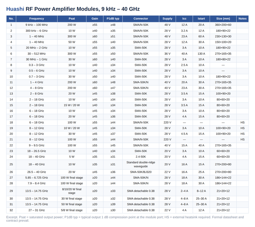
Fig. 1 Huashi 1–40 GHz RF power amplifier modules: 1 W to 200 W saturated power, 30–60 dB gain, SMA-50K / 2.92-K / BJ320 waveguide interfaces (excerpt)
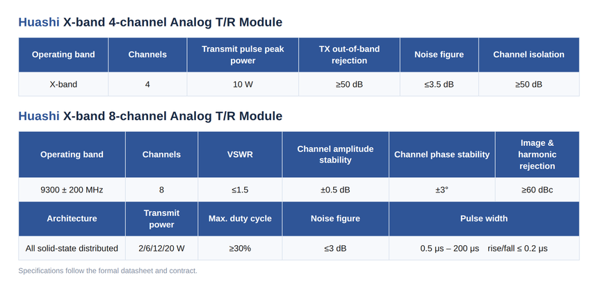
Fig. 2 Huashi X-band 4-channel / 8-channel analog T/R modules: 10 W peak transmit and 2 W to 20 W options, channel isolation ≥ 50 dB
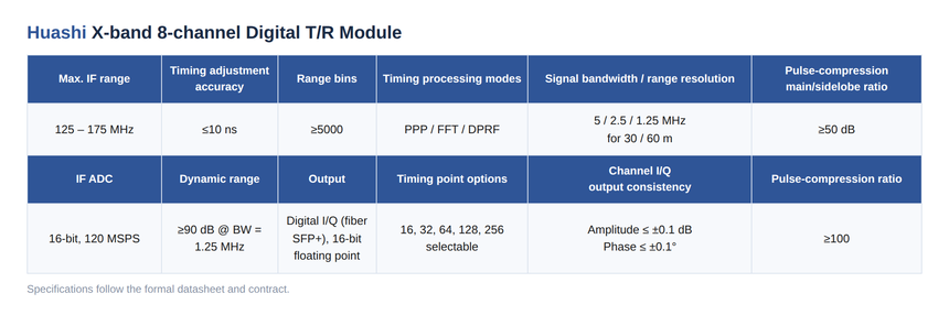
Fig. 3 Huashi X-band 8-channel digital T/R module: 16-bit / 120 MSPS IF sampling, channel I/Q amplitude ≤ ±0.1 dB and phase ≤ ±0.1° The table above lists published ranges and typical values for initial comparison only; specific model, band, power, interface, temperature grade and delivery format follow the formal datasheet and contract. If a project needs 24 GHz wideband conversion, multi-channel T/R or a custom amplifier module, send the band, bandwidth, power, interface and temperature requirements and we will respond with a link-budget-based recommendation. Note: this article records engineering experience. The parameters and criteria are for design discussion and do not constitute an acceptance commitment for any specific product. Any scenario involving transmission, spectrum or airspace use must obtain the appropriate authorization and be tested under authorized conditions. |